Testing a Constructal Climate Model

By Willis Eschenbach

The first rule of climate physics: When in doubt, assume a spherical cow and see how far the joke will take you. In this case, a smooth, two‑zone Earth plus one organizing principle turns out to go a surprisingly long way.

In 2023, I played with Adrian Bejan’s Constructal Law, which states that flow systems far from equilibrium evolve to maximize access to flow. For the climate, this means the system naturally rearranges itself to move as much heat as possible from the hot tropics to the cold poles. Here, the Earth is downgraded to a featureless ball with a hot equatorial belt and cold polar caps, and the only “decision” the system gets to make is how wide that hot belt is when it maximizes poleward heat flow.

The two‑zone sphere

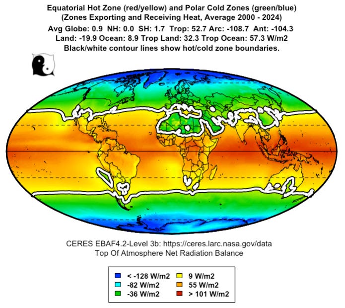
Picture a smooth Earth with lines at ± θ around the equator; between them is the hot belt, and poleward of them are the cold caps. Heat flows from hot to cold, driven by the temperature difference, and the Constructal game is to let θ slide until that heat flow is as large as possible. Figure 1 is the cartoon, and Figure 2 shows the real Earth’s hot and cold zones from the Clouds and the Earth’s Radiant Energy System (CERES) top‑of‑atmosphere radiation balance; despite the missing continents and currents in the model, the real planet organizes into a very similar warm belt and cool caps.

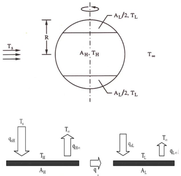
In the hot zone, absorbed solar power is the projected area times the solar constant times one minus the hot‑zone albedo, and emitted power is the area times the sum of one minus the greenhouse fraction times σ times the hot‑zone temperature to the fourth power, with analogous expressions for the cold caps. The difference between absorbed and emitted power in each region is the heat flow q connecting hot to cold. For buoyancy‑driven circulation, Bejan and Reis found that q scales like a conductance C times the temperature difference to the three‑halves power. That leaves five unknowns (hot and cold temperatures, q, the hot‑zone area fraction x, and C) and only three radiative balance equations. As such, the Constructal Law supplies the missing condition: choose x to maximize q, which is the mathematical statement where dq/dx = 0 at the optimum.

In practice, this is a nested optimization. For a given x, solve for temperatures and q. Next, vary x to maximize q, then tune C so that the model’s hot–cold temperature difference matches the observed one. The only external inputs are the hot and cold albedos, hot and cold greenhouse fractions, a single conductance parameter, and small ocean heat‑absorption terms in each zone, all drawn from CERES and related data.

Temperatures, boundary, and heat flow

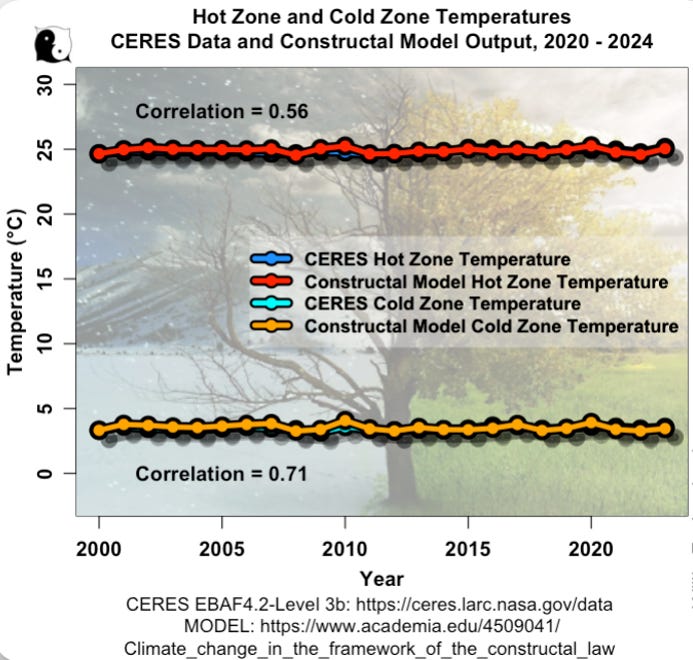
Over 2001–2024, the model gets the mean hot‑ and cold‑zone temperatures within about 0.1°C, tracks the year‑to‑year ups and downs, and captures the slight warming trend, as shown in Figure 3. The modeled swings are a bit larger than observed, but the timing and qualitative behavior match well.

The Constructal solution puts the hot/cold boundary at about 36°N/S, while CERES puts the top‑of‑atmosphere radiation‑balance boundary at around 34°, so the model is off by roughly 2° of latitude, about 220 km. Figure 6 shows that offset, which comes almost entirely from deserts. The Sahara, Arabia, Australia, and the Gobi radiate more than they absorb and so fall on the “cold” side observationally, while the smooth sphere has no deserts and assigns those latitudes to the hot belt.

For poleward heat transport, the modeled peak transport comes out around 14.9 petawatts versus the observed 12.3 petawatts, a global mean excess of about 5 watts per square meter, mostly because of those deserts being misassigned to the hot zone. But the anomalies are where the model shines: Figure 4 shows that the year‑to‑year changes in heat flow match very closely, with a root‑mean‑square error of only 0.04 petawatts, small compared to the natural variability.

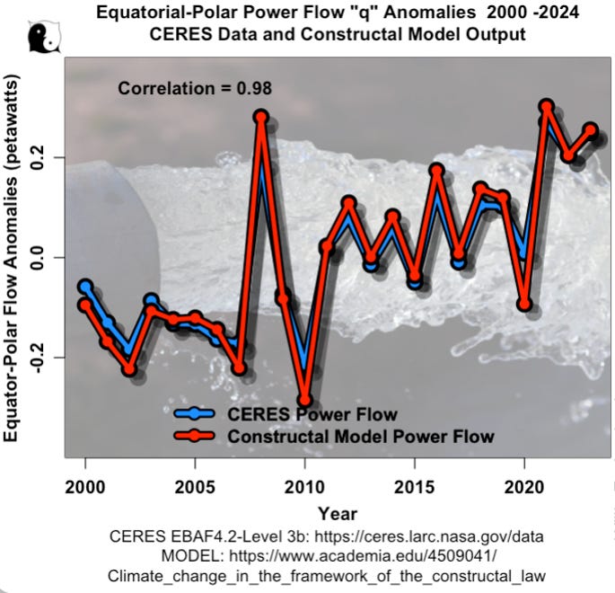
That means that, armed only with annually updated albedo and greenhouse fields and a Constructal optimization, the two‑zone sphere captures the dynamics of how the climate’s heat transport responds to changing radiative conditions.

Climate sensitivity from a smooth ball

To get an equilibrium climate sensitivity (ECS), the model is run with an extra 3.7 watts per square meter of downward flux, the standard forcing for a doubling of CO₂, and then allowed to reoptimize. The hot belt warms by about 1.09°C and the cold caps by about 1.12°C, giving a global mean warming of about 1.10°C. Therefore, the ECS in this framework is roughly 1.1°C per CO₂ doubling. The model omits a whole gallery of emergent negative feedback—thunderstorms, organized deep convection, El Niño/La Niña, tornadoes—that rapidly move heat from the surface into the atmosphere and thus limit surface warming, so the real system is almost certainly less sensitive than this spherical cow.

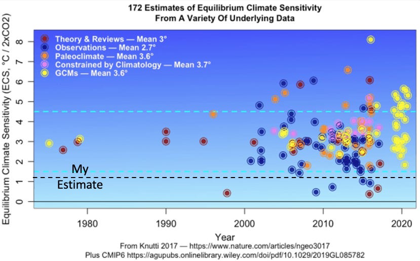
The IPCC’s likely range is 1.5°C to 4.5°C per doubling, so this Constructal result lies below their range but aligns with several observational estimates such as those of Lewis and Curry. Figure 5 shows that the spherical cow sits about the lower, observation‑based estimates rather than the higher model‑based ones.

What the spherical cow is telling us

So, with two zones, four variables, three tuned parameters, and one maximization principle, this ultra‑simple smooth‑sphere model:

• Reproduces hot‑ and cold‑zone temperatures and their interannual variability, including the observed warming trend.

• Gets the hot/cold boundary within a couple of degrees, missing mainly where real‑world deserts sabotage the smooth‑sphere assumption.

• Tracks the temporal structure of poleward heat‑transport anomalies with very low error compared to natural variability.

On top of that, it yields an ECS of about 1.1°C per CO₂ doubling while omitting known negative feedback, strongly suggesting that the real climate sensitivity is modest, not extreme. The broader point is that if you honor basic radiative constraints, feed in real albedos and greenhouse fractions, and let the system maximize its own heat flow, you can capture the central behavior of Earth’s climate with a geometry to which any full‑blown GCM would be embarrassed to admit.

As always, it is not the last word on anything, but it is a useful reminder that the climate behaves like a robust flow system—not a delicate piece of clockwork forever on the brink of collapse—and that even a spherical cow can tell you that much.

About the Author: Willis Eschenbach is a retired generalist without significant credentials of any sort. His life’s motto has been “Retire Early … And Often”. As a result, he has worked at almost every job known to man—cowboy, musician, commercial fisherman, CFO of a $40 million/year company, shipyard manager on a remote South Pacific atoll, author, consultant to Peace Corps and USAID, artist, cook, longshoreman, international smuggler, psychotherapist, shoemaker, farm field worker, cabinet maker, gold miner, commercial diver, and many, many more. He is a self-educated polymath whose great-grandfather said “If you have to frame your diploma and hang it on the wall, there was something wrong with your education“.